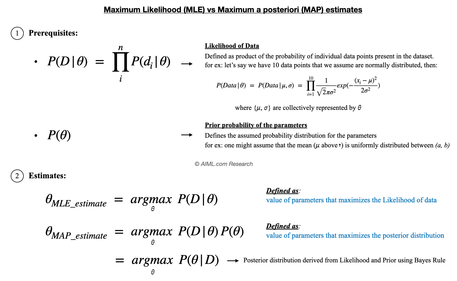
Simply put,
- MLE: estimates of parameters that maximizes the likelihood of data
- MAP: estimates of parameters that maximizes the posterior probability
The following figure explains this in more detail:
MLE vs MAP explained using an Example
Estimating the Bias of a Coin: Suppose we have a coin, and we want to estimate the probability (p) that it lands heads up. We don’t know if the coin is fair, so p could be any value between 0 (always tails) and 1 (always heads).
Let’s assume, we flip a coin 10 times and observe the following outcomes: 7 heads and 3 tails. Then the MLE and MAP estimates would be calculated as follows:
| MLE Estimate | MAP Estimate |
|---|---|
| Concept: In MLE, we want to find the value of p that makes the observed data (7 heads, 3 tails) most likely | Concept: In MAP, we use both the likelihood of the observed data, as well as our prior belief about p Prior belief: Let’s assume we have a prior belief that the coin is likely to be fair. This belief can be represented as a prior distribution for p, by a Beta distribution which peaks at p=0.5, when used with parameters α=2 and β=2 (indicating our belief that the coin is likely to be fair). This is represented by p^(2-1) (1-p)^(2-1) |
| Method: The likelihood function for 7 heads in 10 flips is L(p) = p^7 (1-p)^3. The estimate in this case would be the value of p that maximizes L(p) | Method: The posterior distribution is proportional to the product of the likelihood and the prior. In this case, it would be p^7 (1-p)^3 x p^(2-1) (1-p)^(2-1) The goal is the find the value of p that maximizes the above expression |
| Results: The maximum value of likelihood occurs for p=0.7. Likelihood plot below: 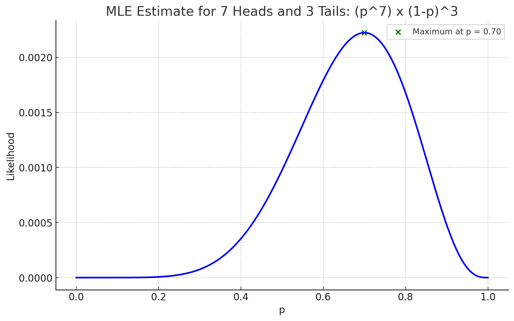 | Results: The maximum value of posterior occurs for p=0.67. Likelihood plot below: 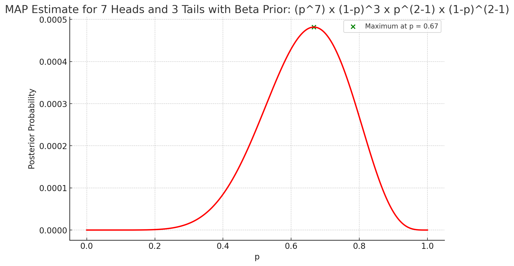 |
| Explanation: The MLE estimate (0.7) only reflects the observed data | Explanation: The MAP estimate would be between 0.5 and 0.7, balancing the observed data with our prior belief in the coin’s fairness |
To conclude, MLE is a frequentist approach focusing solely on the observed data, while MAP is a Bayesian approach that combines data with prior beliefs. The choice between them depends on the specific context, the amount of data available, and whether incorporating prior knowledge is deemed important.
Video Explanation
- In the following video, Prof. Jeff Miller aka. MathematicalMonk explains the differences between MLE and MAP estimates. Even though the video is titled MAP estimates, the video also explains MLE estimates, and contrasts it with MAP estimates.

