As linear regression is meant to provide a modeling framework for stochastic phenomena, there is always going to be some degree of variability inherent in the model estimates produced. While what is considered “good” for a regression model must be evaluated in the specific context of the modeling situation, in all cases, lower variability, or more precise estimates of model coefficients, is desired. Even if a model produces accurate results on average, if it comes with high variance, there would be significant risk from using such a model. Presenting below are a few measures used to estimate the variability in linear regression model:
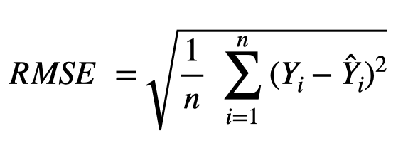
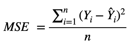
Root Mean Squared Error (RMSE)
The root mean-squared error is the square-root of the average of the sum of squared residuals across all data points. The formula for the RMSE is as follows:
We will use the example dataset given in the table below to break down RMSE into different components. After the model is fit, the residuals are calculated by subtracting the model predictions (![]() ) from the actual values of the dependent variable (Y) for each observation. In order to ensure that the positive residuals do not cancel out the negative residuals, the residuals are squared. Another advantage of taking the square is to penalize excessively large residuals, such as the last observation of this data set. The squared residuals are then summed up, which in this example, would add up to 46, and then divided by the number of observations (5) to get the mean-squared error (46/5 = 9.2). Finally, the square root is taken to arrive at the RMSE (3.03). The square root function is applied at the end to convert the measure back to the original scale of the data, since the residuals were squared before being summed up.
) from the actual values of the dependent variable (Y) for each observation. In order to ensure that the positive residuals do not cancel out the negative residuals, the residuals are squared. Another advantage of taking the square is to penalize excessively large residuals, such as the last observation of this data set. The squared residuals are then summed up, which in this example, would add up to 46, and then divided by the number of observations (5) to get the mean-squared error (46/5 = 9.2). Finally, the square root is taken to arrive at the RMSE (3.03). The square root function is applied at the end to convert the measure back to the original scale of the data, since the residuals were squared before being summed up.
| Actual value, Y | Predicted value, Y_hat | Residual (Y - Y_hat) | Residual (Squared) |
|---|---|---|---|
| 10 | 8 | 2 | 4 |
| 15 | 19 | -4 | 16 |
| 13 | 14 | -1 | 1 |
| 12 | 12 | 0 | 0 |
| 20 | 25 | -5 | 25 |
Lower RMSE is obviously desired, as it represents less variability across the model’s predictions. Making any assessment on whether the model fit is “good” based on the value of RMSE is dependent on the scale of the original data. One way to add context is to compare the average of the original data (Y) with the RMSE value. In our example above, the average of the data is 14 compared to an RMSE of 3.03, which gives some evidence that the variability is lower relative to the scale of the data compared to if the RMSE was say 10. However, it is always recommended to evaluate using multiple criteria to understand the variability, and certain metrics might be more applicable to some data contexts compared to others.
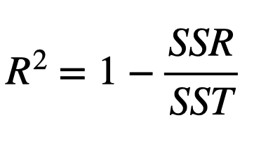
Coefficient of Determination (R2)
The R2 is another commonly used metric to evaluate the fit of a linear regression model. In terms of variability, R2 is a ratio of the total variation in the dependent variable (Y) that is explained by the predictors (X) included in the model. The formula for calculating R2 is:
Unlike RMSE, which has no upper bound, R2 always ranges between 0 and 1, where higher values indicate that a higher proportion of the variability is accounted for by the model. In the extreme cases, an R2 of 0 implies that the predictors provide no value to the model beyond what would be obtained by simply taking the average of the target variable across all observations. On the other hand, an R2 of 1 indicates a model that perfectly explains all of the variability present in the target variable.
Let’s extend the same dataset used in the RMSE example above to calculate R2.
| Actual value (Y) | Predicted value (Y_hat) | Residual (Y - Y_hat) | Residual Squared (SSR) (Y - Y_hat)^2 | Difference from average (Y - Y_avg) | Total Sum of Squares (SST) (Y - Y_avg)^2 |
|---|---|---|---|---|---|
| 10 | 8 | 2 | 4 | -3 | 9 |
| 15 | 19 | -4 | 16 | 2 | 4 |
| 13 | 14 | -1 | 1 | 0 | 0 |
| 12 | 12 | 0 | 0 | -1 | 1 |
| 20 | 25 | -5 | 25 | 7 | 49 |
Here the difference between the actual values (Y) and the overall average (![]() ) must be calculated for each observation, squared, and summed up, just like was done for the residuals. In this example, the calculation, which is called the Total Sum of Squares and denoted SST (last column in the above table), results in a value of 63. This is compared to the Residual Sum of Squares (SSR) of 46, which was computed above. Plugging these into the formula for R2 produces a value of .27, implying that 27% of the total variability in the Y variable was accounted for based on the model used.
) must be calculated for each observation, squared, and summed up, just like was done for the residuals. In this example, the calculation, which is called the Total Sum of Squares and denoted SST (last column in the above table), results in a value of 63. This is compared to the Residual Sum of Squares (SSR) of 46, which was computed above. Plugging these into the formula for R2 produces a value of .27, implying that 27% of the total variability in the Y variable was accounted for based on the model used.
SSR = 4 + 16 + 1 + 0 + 25 = 46
SST = 9 + 4 + 0 + 1 + 49 = 63
R2 = 1 – (SSR / SST) = 1 – (46 / 63) = 0.27
Adjusted R2
If the model includes more than one predictor variable (X), an adjusted R2 statistic is more appropriate to use, as it includes a penalty for additional predictors that are not useful in reducing model variability. As more predictors are added, the regular R2 can only increase compared to a model with fewer predictors, even if the new variables provide no value. The formula for adjusted R2 is as follows, where k refers to the number of predictors in the model, and n is the sample size.
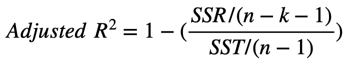
If k = 1, the denominator of the second term reduces to just n, and after expanding the numerator and performing some algebra, the entire right side reduces to the original R2.
Global F-Test
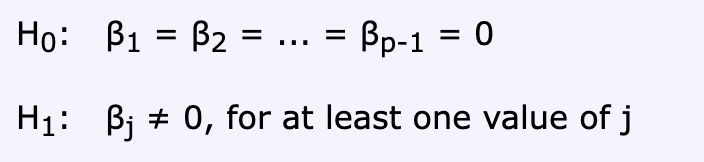
The Global F-Test is a hypothesis test of whether the collection of predictor variables used in a regression model provides any capability in explaining the variance in the target variable compared to a model without any predictors.
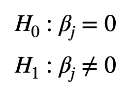
The setup of the test consists of the null hypothesis (H0) that all of the model coefficients are 0, meaning the entire set of predictors adds no explanatory value; whereas the alternative hypothesis (H1) is that at least one of the predictors’ coefficients is not equal to 0, or has statistical significance.
Thus, a small p-value that would result in a rejection of the null hypothesis could potentially indicate that the model has some value, but it does not directly give insight into which individual predictors are most statistically significant.
Hence its name, the Global-F test is based on the F-distribution, which is a statistical distribution formed by the ratio of two independent chi-squared distributions. The formula used in this test is a function of the ratio of the regression sum of squares (SSR) to the residual sum of squares (SSE), with each divided by its respective degrees of freedom.

The result of this ratio produces the test statistic, which is compared against the critical value of the F distribution with the same degrees of freedom in order to determine its significance. From a conceptual standpoint, the ratio can be thought of as a signal-to-noise ratio, meaning that if SSR is large compared to SSE, the model produces a lot of signal compared to noise, or variability, resulting in a large F-statistic and thus a low p-value, which is good and desirable. On the other hand, if SSR is small or close relative to SSE, the noise is greater than the signal, thus producing a low F-statistic and high p-value, thereby indicating poor model fit.
While the Global F-test is an easily interpretable metric that is useful as a first glance in evaluating the fit of a model, it should be used in conjunction with other variability measures as well as detection techniques to validate the assumptions of a regression model.
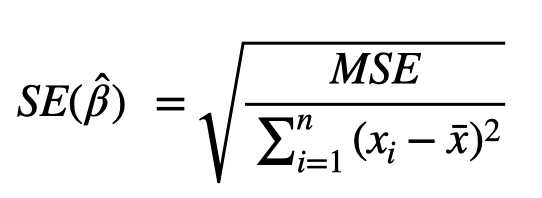
Standard Errors
While the metrics discussed so far are used to evaluate a model’s variability at the macro level, it is usually also of interest to quantify the variance of the individual predictors. The classical setup for measuring the variability of a regression coefficient is to use the standard error and t-test. The standard error is analogous to a standard deviation measure that could be computed from any sample of data, and in the regression context, is computed for each coefficient by the following formula, where MSE is the mean squared error, referring to the variability of the overall model, and the denominator is measuring the variability of a single predictor variable, where ![]() represents the average of x values for the coefficient being evaluated.
represents the average of x values for the coefficient being evaluated.
where,
Thus, the standard error is high when the model variability is large relative to the predictor’s variability.
t-test for individual predictors
In order to understand the significance of individual model coefficient, we perform the t-test. As given below, the null hypothesis is that the jth model coefficient is 0, and the alternate hypothesis is that the model coefficient is not equal to 0. Degrees of freedom is n – p – 1 where p is the number of predictors in the model.
The t-statistic is computed using the ratio of the estimate for the coefficient over the standard errors as follows:
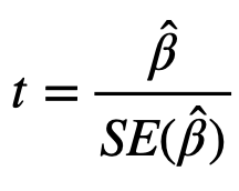
The result of this ratio produces the test statistic, which is compared against the critical value of the t-distribution with the same degrees of freedom in order to determine its significance. It should be noted that the t-statistic is large when the standard error is small. Thus, the standard error can be thought of as a measure of precision for the estimated coefficient.
