What are some of the most common feature engineering techniques?

Introduction

Feature Engineering is the process of preparing data for modeling. It involves combining existing features, creating new features based on domain knowledge, or transforming features to make them more suitable for a particular algorithm. It is a crucial step in the machine learning pipeline, as the quality of the features used can significantly improve the prediction accuracy and generalization of the model. Various techniques used in feature engineering are as follows:

1. Dummy encoding: In order to represent a categorical variable in a machine learning model, it usually must be somehow coded numerically before it is used in the training of a model. The easiest way to do so is to create a series of dummy variables (k-1 dummies for a variable with k distinct categories) that take on a value of 1 when the original field is equal to the kth category and 0 otherwise. As one level can be represented when all of the dummy variables are set to 0, there should be one less dummy variable compared to the total number of unique categories of the variable to avoid redundancy. An illustration of dummy variable transformation is shown below, assuming the four categories for country are the only unique values present in the dataset. 
   
   Dummy encoding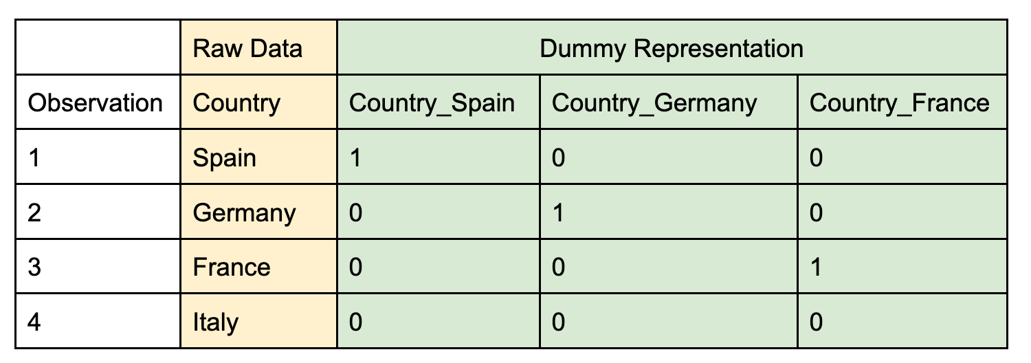
   
   
   
2. One-hot encoding: This technique is used to represent categorical features as binary vectors. Each category is represented by a binary vector where one element is set to 1 and the rest are set to 0. This allows the machine learning algorithm to better handle categorical features.

3. Ordinal Encoding: This is another way to convert a categorical variable into a numeric representation suitable for model training. Unlike dummy encoding, ordinal encoding requires knowledge of the target values corresponding to each observation. It works by sorting the original data in ascending order by the values of the target and then replacing the raw values with the index of the sorted data. An advantage of ordinal encoding is that it creates a monotonic relationship between the transformed input variable and target, which is beneficial for some algorithms. It is important to obtain the mapping from the original to transformed version of the variable using only the training data to avoid information from the test set leaking into the training process and possibly inducing bias.
   
   Ordinal Encoding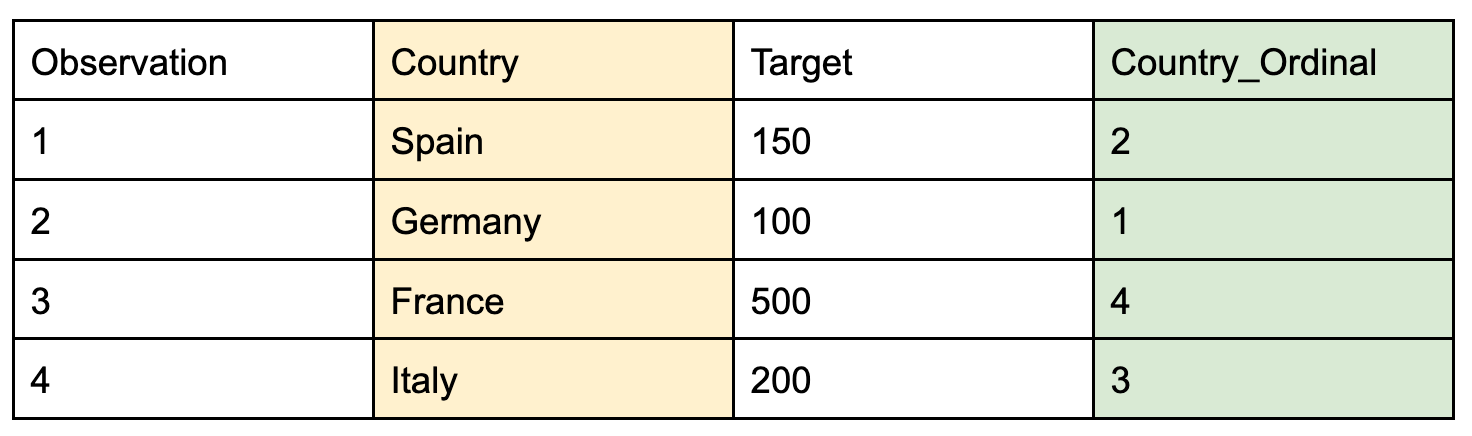
   
   
   
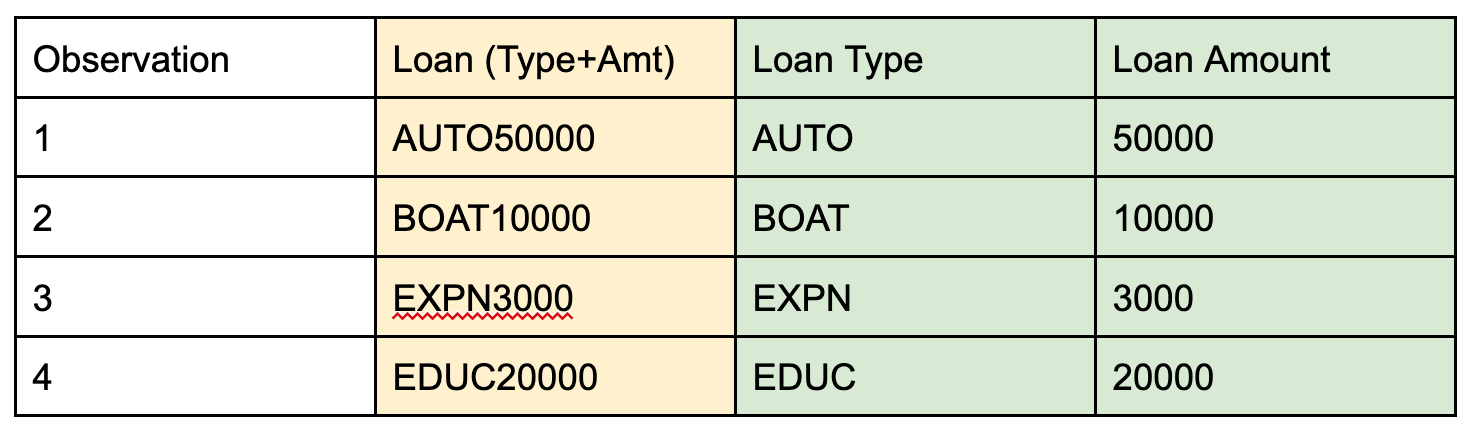
4. Text Feature Extraction: In some text fields, especially those that follow a consistent pattern throughout all of the observations, features can be extracted based on sub-components of the original text strings. In the example below, the original field contains a combination of the type and amount of a loan in the same string. Using text mining and regular expressions, the loan type can be found by extracting the first four characters of the string, and the amount by extracting separately everything after the fourth position. Note that one of the categorical encoding methods described previously would need to be applied to the Loan Type field before using it in a model.
   
   Text Feature Extraction
   
   
   
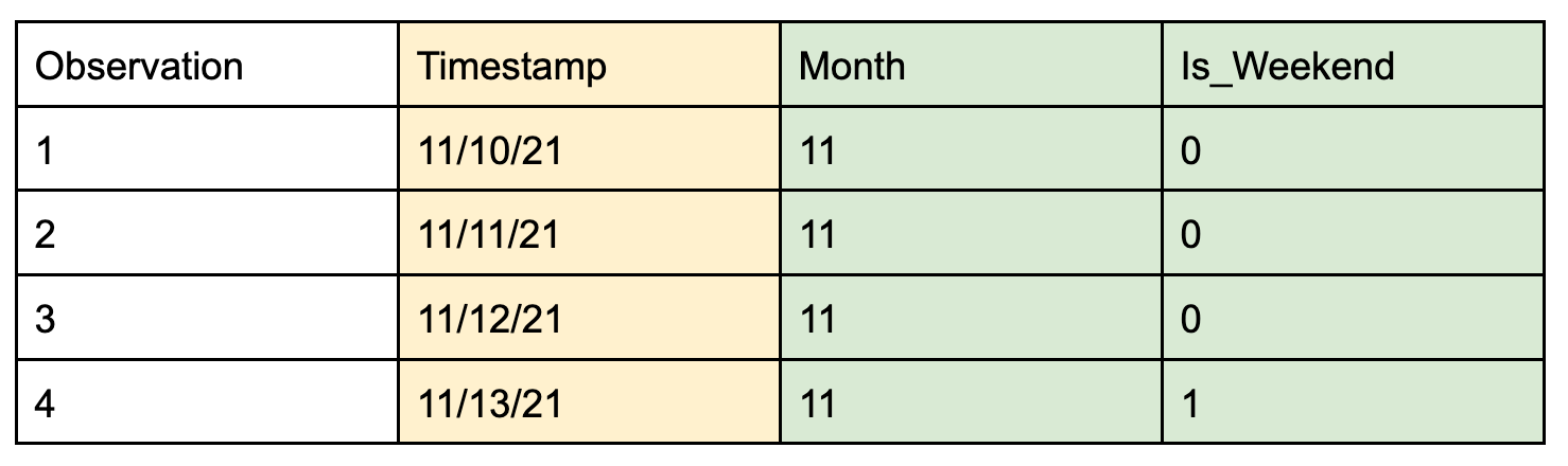
5. Date Extraction: Timestamp attributes can be very informative for certain forecasting applications. A common feature engineering technique that allows one to utilize information from these types of features is to extract components from a timestamp, such as the year, month, day, or hour. More complicated dimensions such as whether the day is a weekend, holiday, or business day can also be highly predictive in certain contexts, such as sales. 
   
   Date Extraction
   
   
   
6. Discretization: Discretization refers to the process of binning a continuous variable into a discrete number of buckets. In some machine learning algorithms, the performance can be improved by using this kind of representation, especially if there are outliers on the original scale of the variable that cause its distribution to be skewed. There are several different techniques that can be used to discretize a continuous variable, and some of the most common are listed below:
   • Equal frequency bins: This technique creates buckets that contain a roughly equal number of observations in each bin. An advantage of this approach is that it creates a balanced distribution out of the new categories created. However, it does not guarantee that the spacing between endpoints is even in the same manner.
     
   • Equal width bins: This technique works similarly to equal frequency bins, but now, the spacing between endpoints of each bin is roughly equal. However, the number of observations falling into each bucket is no longer constrained, so some buckets might contain very few data points. 
     
   • Decision Tree discretization: This method fits a decision tree using the candidate variable as input and the target as the output. The splits it creates during the construction of the tree form the endpoints of the discrete version of the variable, and the actual values for the derived variable are usually the average values of the target at each node of the decision tree. This technique provides the advantages that using a decision tree in a supervised learning context does, but unlike the previous two methods, it does require utilizing the target variable in the discretization process. 
     
   • Subject Matter Knowledge: Depending on the context of the problem, domain knowledge might be more beneficial than a quantitative technique in determining how to create buckets. Ultimately, most data science projects are only useful if they are applied in an appropriate context that derives benefit to the stakeholders.
     

7. Feature scaling: Some machine learning algorithms are sensitive to the scale of the features, so it is often useful to scale the features to a common range, such as [0, 1] or [-1, 1]. This can be done using techniques such as min-max scaling or standardization.

8. Feature creation: This involves creating new features using existing ones based on domain knowledge. For example, if we have a dataset of customer transactions, we can create new features such as average amount spent per purchase, days since last purchase, maximum purchase amount etc.