Source: Understanding LLM Decoding Strategies
Introduction
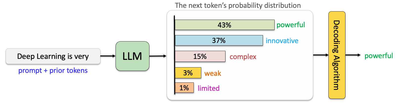
Large Language Models (LLMs) are auto-regressive models that predict the next word (or token) by calculating probabilities for a sequence of previous words based on their training data. These probabilities are then decoded to generate text. Various decoding strategies exist for next-word prediction. This post explores these approaches, compares their behavior, and demonstrates how LLMs allow customization through parameters like temperature. But before getting to that, let’s understand some important concepts first.
Auto-regressive model
Auto-regressive (AR) models are a class of models that generate output sequentially by predicting the next element in a sequence based on the previous elements. In the context of language models, an AR model generates text one token at a time, using all the tokens generated so far as input for the next prediction.
Decoding of Token Probabilities
Language models predict the next token by processing input text through a series of steps. First, the input is tokenized and mapped to embeddings, which are then passed through the transformer decoder. The decoder uses self-attention and feed-forward layers to generate a contextualized sequence representation. This representation is projected through a linear layer into the vocabulary space, producing logits for each token. Applying a softmax activation converts these logits into a probability distribution, with each value representing the likelihood of a token being the next in the sequence. Finally, the decoding process determines which token to select based on the probability distribution.
Common Approaches for Next-Word Prediction
Greedy Search
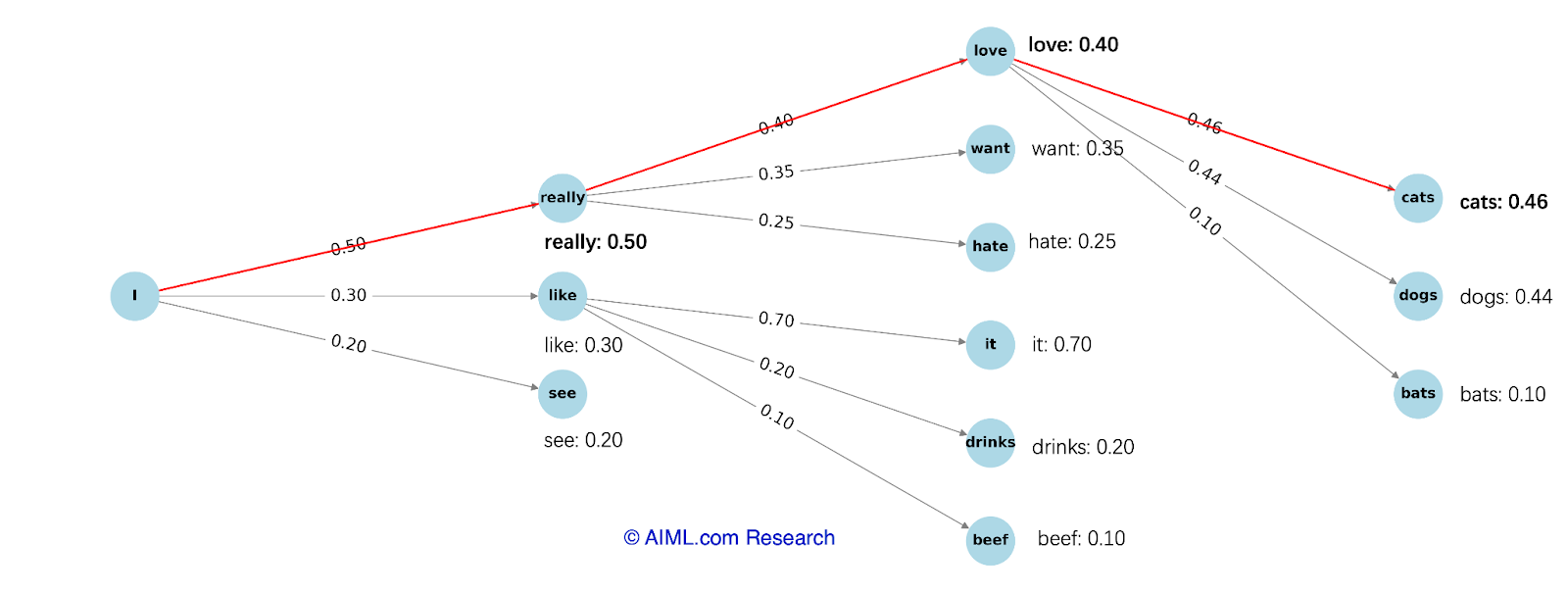
Greedy Search is a decoding method where, at each step, the model selects the token with the highest probability. This straightforward approach ensures that the output is deterministic and coherent in many cases. However, it often struggles with generating diverse or creative responses, as it follows the most likely path without exploring alternatives. This can lead to repetitive loops or suboptimal outputs, especially in tasks requiring nuanced or imaginative answers.
As depicted in the figure below, the model selects the highest probability token at each step with greedy search decoding, resulting in the sequence “I really love cats.” Note that even though the last word choice “cats” and “dogs” have similar token probabilities, it will always generate “I really love cats”
Source: AIML.com Research
Beam Search
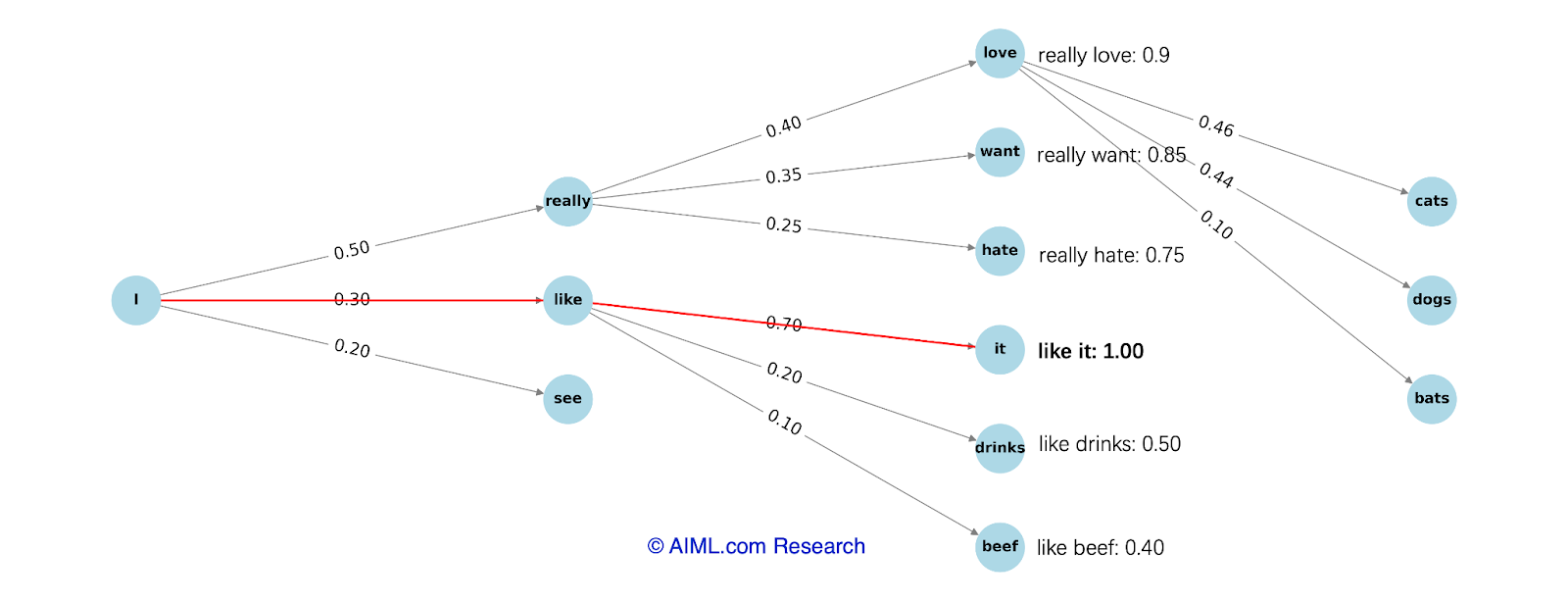
Beam Search is a decoding strategy that simultaneously explores multiple candidate sequences (referred to as beams) rather than selecting tokens step by step like greedy search. At each step, it keeps the top sequences with the highest cumulative probabilities, ultimately choosing the one with the highest overall probability. This method improves coherence and diversity compared to greedy search, as it evaluates a broader range of possibilities. However, beam search can be computationally expensive and may still generate repetitive or overly generic outputs, particularly in tasks requiring more creativity or specificity.
As shown in the figure below, this is a beam search with a beam width of 2. It selects the sequence with the highest cumulative probability among two candidate sequences. In this example, the chosen sequence is “I like it.”
Source: AIML.com Research
Sampling
Sampling is a decoding method that introduces randomness by selecting the next token based on its probability distribution rather than always choosing the most likely one. This approach allows for more creative and diverse responses, making it particularly suitable for tasks like storytelling or creative writing. However, the randomness in sampling can lead to incoherent or less relevant outputs, especially if the probabilities for lower-quality tokens are not sufficiently suppressed.
Example:
Given the probability distribution for the next word:
{“happy”: 0.5, “excited”: 0.3, “sad”: 0.2}
Sampling might choose “excited” or “sad” instead of the most likely token “happy”, introducing variability to the response.
Top-K Sampling
Top-k Sampling is a decoding strategy that restricts the selection pool for the next token to the top k highest-probability candidates, effectively filtering out less likely words. Sampling is then performed within this reduced set, introducing controlled randomness while maintaining coherence. This method balances creativity and reliability, making it well-suited for tasks like dialogue generation or creative writing. However, the choice of the k value is critical; a small k can limit diversity, while a large k may reintroduce incoherence.
Example:
For the probability distribution:
{“happy”: 0.5, “excited”: 0.3, “sad”: 0.2, “angry”: 0.05, “confused”: 0.02}
If _k = 3_, the pool is reduced to:
{“happy”: 0.5, “excited”: 0.3, “sad”: 0.2}
Sampling is then performed within this set, ensuring the model avoids unlikely tokens like “angry” or “confused” while still allowing variation in its output.
Top-P (Nucleus) Sampling
Top-p (Nucleus) Sampling is a decoding method that dynamically selects the smallest set of tokens whose cumulative probability exceeds a specified threshold (p). Unlike top-k sampling, which fixes the number of candidates, top-p adapts the pool size based on the distribution, ensuring that only the most probable tokens are considered while still allowing for diversity. This approach provides flexibility and helps balance coherence and creativity. However, careful tuning of the _p_ value is necessary to avoid overly random or overly generic outputs.
Example:
For the probability distribution:
{“happy”: 0.4, “excited”: 0.3, “sad”: 0.2, “angry”: 0.05, “confused”: 0.05}
If p = 0.7, the pool is:
{“happy”: 0.4, “excited”: 0.3}
The cumulative probability of 0.7 is reached with these two tokens, and sampling occurs only within this set, excluding less likely options like “sad” or “angry.”
Strategy for Controlling Next-Word Prediction in LLMs
One of the most common and effective strategies for controlling next word prediction in LLMs is Temperature
What is Temperature?
Temperature is a parameter that adjusts the randomness of a model’s predictions by scaling the logits before applying the softmax function. A higher temperature (e.g., 1.0) flattens the probability distribution, making the model more likely to sample less probable tokens, resulting in more random and diverse outputs. Conversely, a lower temperature (e.g., 0.2) sharpens the distribution, increasing the likelihood of selecting the most probable tokens, leading to more deterministic and focused outputs.
The temperature typically ranges from 0 to 1, though it can be set higher for experimental scenarios. Commonly used values are between 0.7 and 1.0 for creative tasks (e.g., story generation) and around 0.2 to 0.5 for tasks requiring deterministic outputs (e.g., summarization or code generation).
The formula for applying temperature in a model’s predictions can be written as:
where:
- $P_i$ : Probability of selecting token $i$ .
- $z_i$ : Logit (raw score) for token $i$ .
- $T$ : Temperature parameter.
- $N$ : Total number of tokens in the vocabulary.
Explaining the concept of Temperature using an example:
For the logits {happy: 2.0, excited: 1.5, sad: 1.0}, applying different temperature values results in varying distributions:
- Temperature = 1.0:
Probability distribution: {happy: 0.42, excited: 0.32, sad: 0.26}
The output is diverse and may select “excited” or “sad” more frequently.
- Temperature = 0.2:
Probability distribution: {happy: 0.85, excited: 0.10, sad: 0.05}
The output is highly focused, almost always selecting “happy.”
Use Cases of Different Decoding Methods
Different decoding strategies are suited to different scenarios. The table below outlines some examples of scenarios where each decoding strategy is most appropriate.
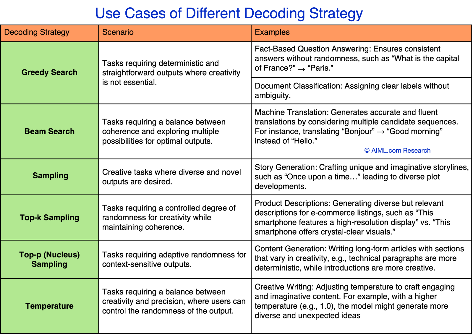
Source: AIML.com Research
Other Novel Decoding Method
In addition to the commonly used decoding methods mentioned above, there are some novel approaches designed specifically to help reduce hallucinations. Below, we introduce a few of these methods.
DoLa: Decoding by Contrasting Layers
Some interpretability studies on large models have shown that in Transformer-based language models, earlier layers encode “low-level” information (such as part-of-speech tags), while later layers capture more “high-level” semantic knowledge. The primary inspiration behind DoLa’s approach to reducing hallucinations lies in emphasizing the knowledge in higher layers while de-emphasizing information from lower layers.
As illustrated in the example, when predicting the next token, the most appropriate choice is “Olympia.” However, if we only consider the final layer, the model might still assign a high probability to “Seattle.” In such cases, while “Seattle” maintains a relatively high probability across all layers, leveraging the contrast between different layers can significantly increase the probability of the correct answer, “Olympia.”
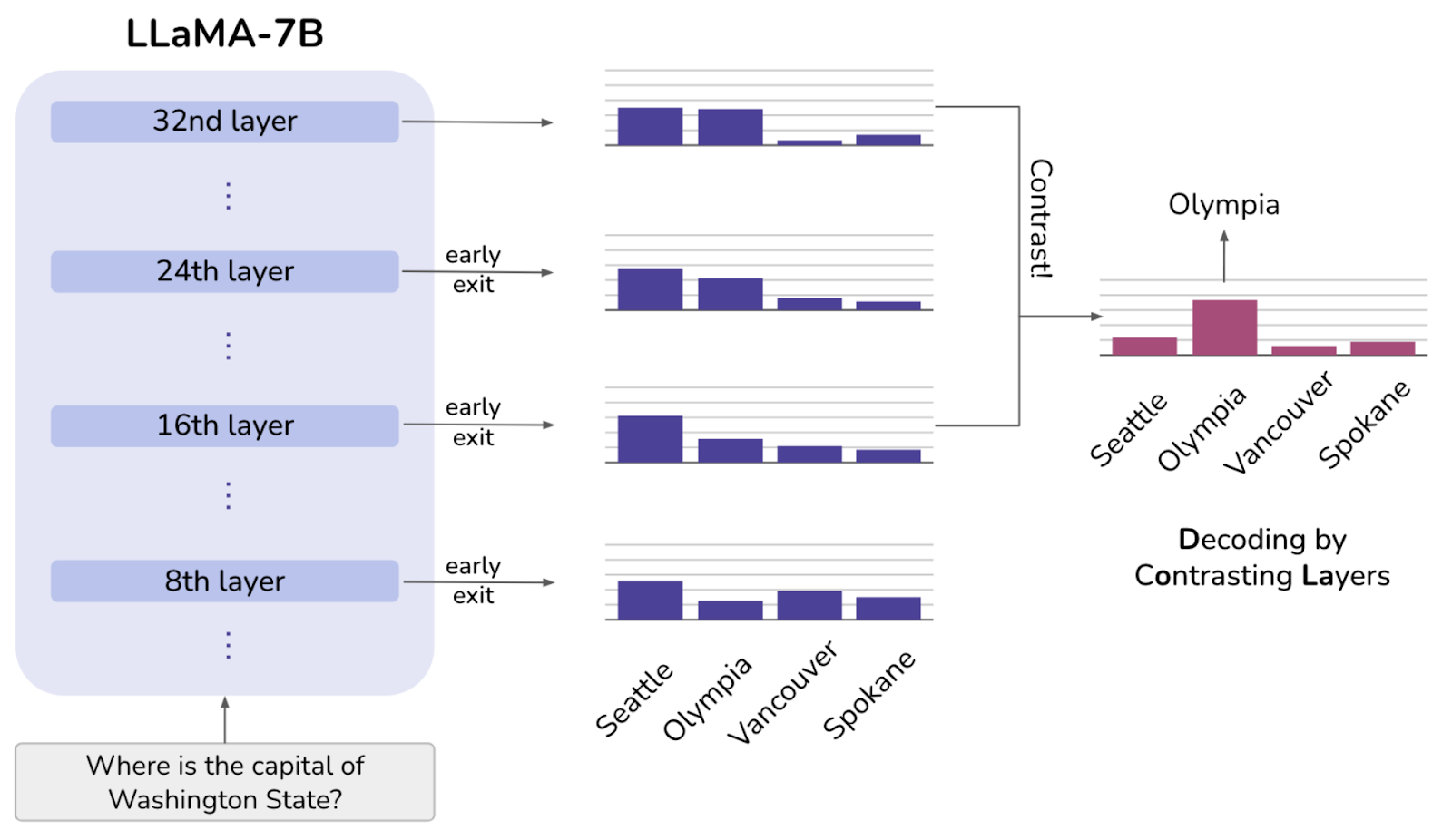
Source: DoLa: Decoding by Contrasting Layers Improves Factuality in Large Language Models by Chuang et al.
The paper also provides specific formulas on how to implement contrastive analysis of token probabilities across different transformer layers, enabling the effective identification of the most preferred answer. For more details, please refer to the original paper.
VCD: Visual Contrastive Decoding
VCD decoding is a simple, training-free method designed to reduce hallucinations in vision-language models. As shown in the Figure, it works by contrasting the token distributions generated from the model when given original visual inputs versus distorted visual inputs. This contrast helps identify and filter out tokens likely to be hallucinations. For more details, refer to the original paper.
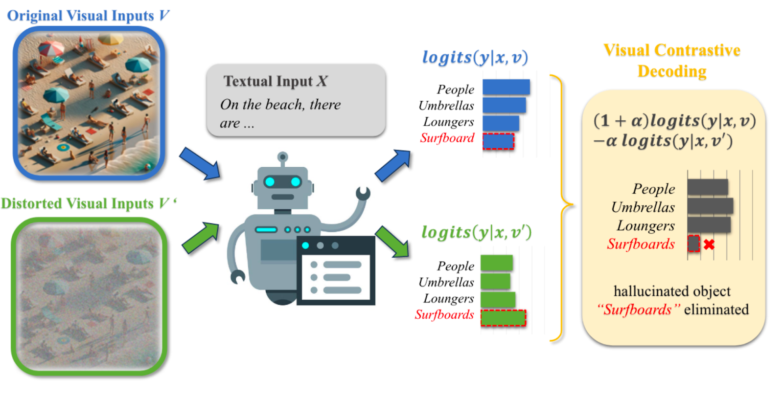
Source: Mitigating Object Hallucinations in Large Vision-Language Models through Visual Contrastive Decoding by Leng et al.
Video Explanation
- The video by Andrew Ng provides a detailed explanation of the beam search algorithm.

- The CS224N lecture on Natural Language Generation provides an overview of decoding techniques for language models, including various sampling methods such as top-k and top-p sampling:
Youtube link: Stanford CS224N NLP with Deep Learning | 2023 | Lecture 11 – Natural Language Generation
Related Questions:
