Linear Model Assumptions
While linear regression is considered to be one of the most simple and interpretable statistical modeling approaches, in order to have confidence in its results, there are several assumptions that must be checked and verified. The most essential ones are the following:
- Independence of errors
- Normality of residuals
- Constant Variance (Homoscedasticity)
- Linearity
- No Perfect Multicollinearity
Let’s delve into each of these assumptions in detail below:
1. Independence of errors
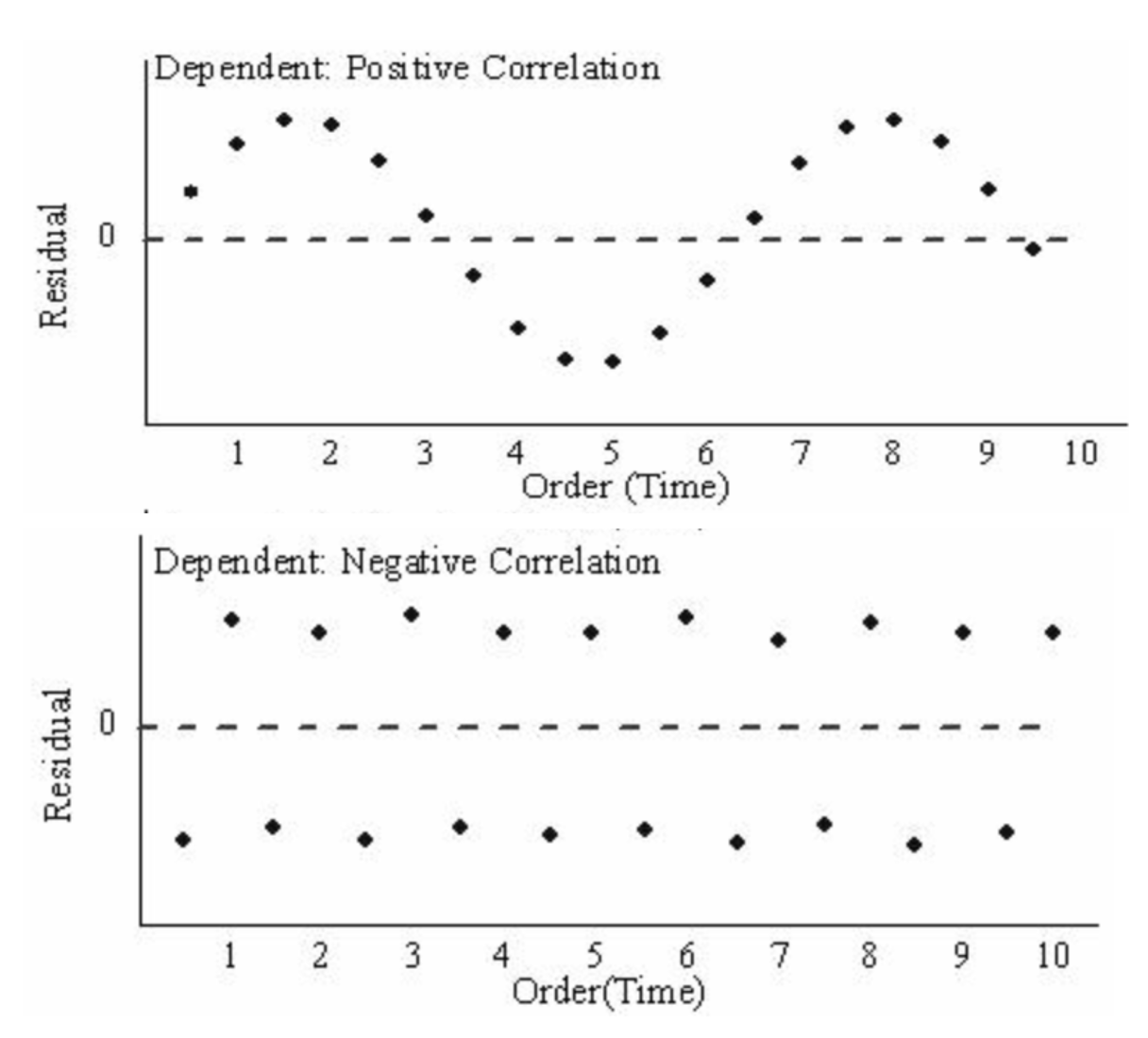
The residuals, or difference between actual and predicted values for each observation, are assumed to be independent of one another. The only way to guarantee the observations are sampled independently is to have knowledge and control over the study design, but as a proxy, a simple plot of the residuals plotted over time can be examined for any noticeable trends that might indicate whether autocorrelation, or temporal dependence, is present.
The following example of a Residual vs. Time plot shows no apparent pattern, which is a good indication that there are no issues with autocorrelation.
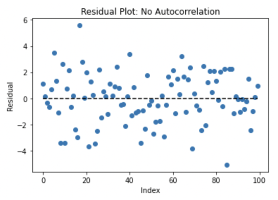
In contrast, if there is a trend observed over the order of the residuals, such as if they tend to follow each other or alternate between being above and below 0, that could indicate a violation of the independence assumption.
If it is believed that there is autocorrelation present in the data, the correlation structure would need to be examined in greater detail. If the issue cannot be isolated to any particular variable or aspect of the data collection process, more specific time series techniques designed to model autocorrelation might be better suited to the data than traditional linear regression.
2. Normality of residuals
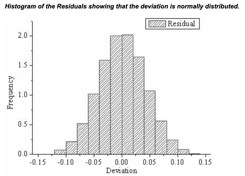
This assumption implies that the errors are identically distributed instances taken from a normal distribution centered at 0. If the residuals were plotted on a histogram, they should follow a bell-shaped curve that peaks at 0 with few observations in the far tails of the distribution as shown below.
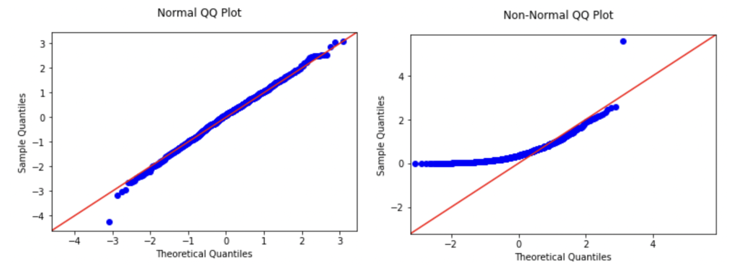
Alternatively, this assumption can be verified using a QQ-plot, on which the points should fall close to the 45-degree line passing through the origin. If the points deviate from that line or follow a different pattern from a straight line, it might indicate a violation of the normality assumption. The first plot below shows an example of data that likely satisfies the normality, where the second would indicate a likely violation.
There are also some statistical tests, such as the Shapiro-Wilk and Kolmogorov-Smirnov, that can be used to assess normality within the framework of a hypothesis test and p-value. The null hypothesis is that the distribution is normal, so if the p-value from one of these tests is less than the chosen significance level, the statistical conclusion would be to reject the null hypothesis and thus the assumption of normality. However, in many real-world datasets that contain a large number of observations, these tests are overly powerful and often detect significance based on sample size alone. Thus, examining the residuals visually through a histogram and/or QQ plot is usually a more practical approach to validating the normality assumption.
If it is determined that there are issues with normality, the most common way to address it is through a transformation of the dependent variable. The Box-Cox or Yeo-Johnson transformations provide an optimization approach using power-based transformations.
3. Constant Variance (Homoscedasticity)
The assumption that the residuals exhibit constant variance across the observations forms the third and final component of the term iid (independent, identically distributed) that is often used in statistics. For all levels of the independent variable(s), the spread of the residuals should be relatively constant. If the variance is non-constant, that would indicate that the model’s predictions are less precise for certain ranges of the predictor variable(s) than others. If the variable is categorical, such as an indicator for male or female, it could be the case that the model predicts with more precision for certain levels of the variable compared to others.
This assumption can be checked by plotting the fitted values of the regression on the X-axis against the residuals of the model on the Y-axis. Any discernible pattern on the residuals vs. fits plot could indicate a violation, and common patterns include fanning out, where the variance increases as the fitted values get larger, or caving in, where the variance is high for both large and small fitted values but smallest in the middle. Below is an example of a properly-looking Residuals vs. Fits plot (left) as well as one that might indicate heteroskedasticity, or non-constant variance (right).
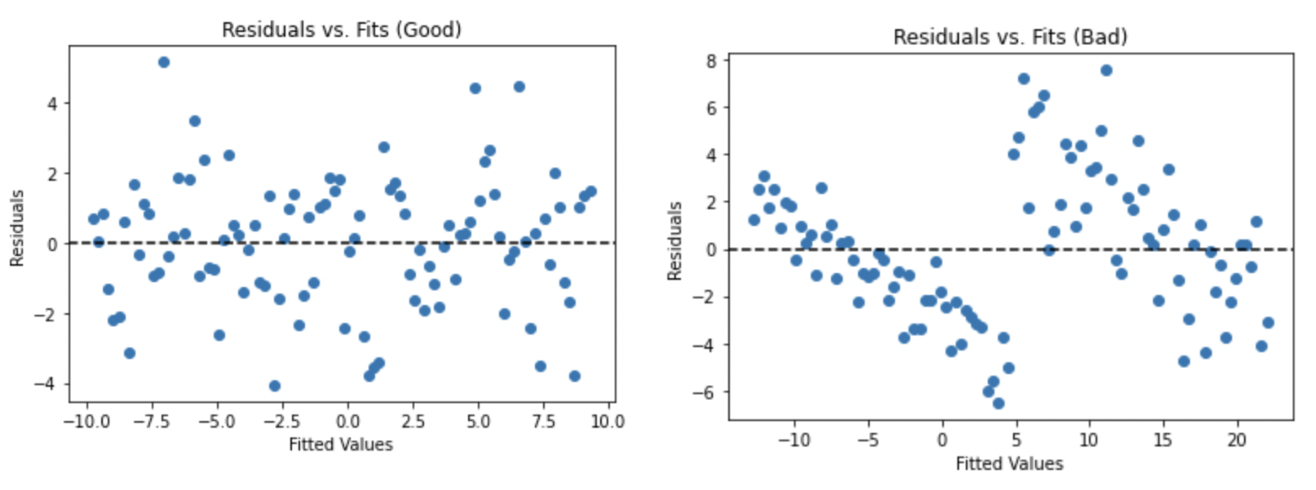
If the assumption does not seem to hold, the most common solution is to transform the dependent variable using a logarithmic or power transformation.
4. Linearity
This assumption requires that the relationship between each predictor variable and the outcome is linear. If the relationship is non-linear on the original scale of the predictor, the variable might need to be transformed so that a linear relation is achieved. This condition is most effectively checked by plotting the data, such as creating scatterplots of each X vs. the Y variable.
If the linearity assumption is violated, the regression model will likely be misspecified and suffer from poor fit and high bias. If a linear relationship cannot be created between the X variables and the target, linear regression would not be a suitable technique, and instead, non-linear models such as ensemble algorithms or deep learning might be better suited for the data.
5. No Perfect Multicollinearity
Multicollinearity occurs when there is very high correlation among two or more of the predictor variables. If one predictor is a linear function of another, it is a case of perfect multicollinearity, and the model is not able to find estimates. In the following example dataset, X3 is related to X1 and X2 by the following relation: X3 = X1 + 2 * X2
| X1 | X2 | X3 (X1 + 2 * X2) |
|---|---|---|
| 2 | 6 | 14 |
| 5 | 9 | 23 |
| 10 | 3 | 16 |
| 12 | 2 | 16 |
| 20 | 5 | 30 |
In this case, a regression model estimated using either least squares or maximum likelihood could not produce unique coefficient estimates. In the formula for the estimates of the Beta coefficients produced by either Ordinary Least Squares or Maximum Likelihood Estimation, (X’X)-1X’Y, the X’X matrix becomes singular and thus the inverse cannot be computed, causing the result to be undefined.
Even if there is no perfect multicollinearity anywhere in the feature space, if two or more predictors are very highly correlated, the matrix can still become unstable, thus increasing the variance of the parameter estimates. This implies less precise estimates of the true model coefficients and makes it more difficult to determine which, if any, of the coefficients are statistically significant (reduced power). It also makes interpretation more difficult, especially when trying to distinguish between the effects of the different predictors on the outcome. Finally, the model itself may become unstable, meaning that small changes in value among the features could result in significant changes to the coefficient estimates.
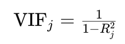
The standard diagnostic for detecting multicollinearity is the variance inflation factor (VIF), which measures how much of the variance of a particular regression coefficient is inflated due to being correlated with other predictors. If the VIF for a variable is larger than 5 or especially 10, it might indicate a problem with multicollinearity. The formula for the VIF is as follows, where the R2 term is the R2 coefficient for the regression of the j-th predictor on all other predictor variables.
Another potential indicator that multicollinearity is present is if the overall F-test is significant, but no individual coefficients show any statistical significance. In severe cases, the signs of the coefficient estimates may even be the opposite of what would intuitively be expected. The most likely scenario in which this occurs is if the correlated predictors have opposite relationships with the target variable, i.e. X1 and X2 are highly correlated with each other, but X1 is positively correlated with the target and X2 is negatively correlated with the same target variable.
If multicollinearity is an issue, a solution is often to remove one of the features that is contributing to the collinearity from the dataset. If it is possible, another potential remedy is to create a derived variable that is a function of each of the variables that are correlated, and then drop the original versions of the variables from the dataset. Finally, a modeling technique that performs built-in feature selection, such as regularized regression or an ensemble method, would be less affected by severe multicollinearity.
Conclusion
Compared to more modern machine learning techniques like decision trees, Random Forest, and Boosting this is one of the perceived drawbacks of linear regression, that it is dependent on several assumptions in order to reliably make use of the results.
