Source: Convolutional layer
About Convolution
Convolution is a mathematical operation that combines two functions (or sets of data) to produce a third function. In machine learning and signal processing, we use convolution to extract features from data, such as images or signals, by sliding a kernel (or filter) over the input.
We can categorize convolution into two main forms: continuous and discrete. In continuous convolution, we integrate functions over a continuous domain, which is commonly applied in areas like signal processing. In contrast, for machine learning and computer vision, we typically perform discrete convolution, representing both inputs and filters as discrete data structures such as arrays or matrices. Thus, discrete convolution becomes the standard operation for feature extraction in modern AI applications. Below, we introduce 1D discrete convolution and multi-dimensional discrete convolution in detail.
1D Convolution
The one-dimensional convolution of an input x[n] and a kernel h[k] is defined as:
In convolution, x[k] is the input signal, and h[k] acts as the filter that transforms the input. Specifically, the convolution operation combines these two by sliding the kernel over the input and computing weighted sums, thereby extracting meaningful features from the input data. The resulting output of the convolution is y[n], which is computed as the operation slides the kernel across the input signal.
Example:
- Input ( x ) [1, 2, 3, 4]
- Kernel ( h ): [1, 0, -1]
Steps:
- First, flip the kernel: [-1, 0, 1]. This flipping step aligns with the definition of convolution, and more importantly, it simplifies the mapping between kernel values and input signal values during the calculation process.
- Slide the kernel over the input and compute the dot product at each position.
Output: y = [2, 2] (assuming valid padding).
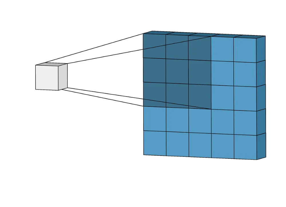
2D Convolution
We can extend the 1D convolution to 2D version, becoming matrix calculation:
Where x[m, n] is the input matrix, h[i, j] is the kernel (filter) matrix of size H \times W , and y[m, n] is the output matrix.
Example:
Input Matrix x:
Original Kernel h:
Steps:
- Flip the kernel (both horizontally and vertically)
- Slide the flipped kernel over the input and compute outputs
For instance, at position (0, 0):
at position (0, 1):
Final Output Matrix:
Please note that in strict mathematical convolution, the kernel is first flipped before being applied to the input. However, in practice, most machine learning and deep learning frameworks (such as PyTorch and TensorFlow) implement cross-correlation instead, thus skipping the flipping step. As a result, these frameworks typically apply the kernel directly without flipping, which makes the operation more computationally efficient.
Convolution in Multiple Dimensions
Similarly, higher-dimensional convolutions (e.g., 3D convolutions) extend this concept to work on volumetric data, such as videos or medical scans. While the process remains fundamentally similar, it now involves sliding a kernel across all spatial and temporal dimensions.
Applications of Convolution
Convolution has diverse applications across various fields. Specifically, it plays a crucial role in areas such as image processing, signal processing, and deep learning. Here are some examples:
- Image Processing: Convolution plays a vital role in tasks like edge detection, blurring, and sharpening. For example, one can detect horizontal edges in a grayscale image by applying a Sobel kernel such as [-1, 0, 1]. In traditional image processing, practitioners manually design kernel values based on mathematical principles. In contrast, deep learning models automatically learn kernel (or filter) values from data during training through backpropagation. This allows convolutional neural networks (CNNs) to discover optimal feature extractors tailored to specific tasks.
- Signal Processing: It is often applied to filter noise from audio or time-series data. For example, a low-pass filter can smooth an audio signal by removing high-frequency noise, improving clarity.
- Deep Learning: Convolution is essential for feature extraction in convolutional neural networks (CNNs). For example, a convolutional layer with a filter like can detect vertical edges in images, aiding tasks like object recognition.
Convolution in Practice
We will look at two examples of Convolution in Practice:
- 1D convolution using a custom kernel in PyTorch
- Defining and using a Convolution layer in a CNN
Example 1:
Here is an example of implementing Convolution using Pytorch on a 1D input:
import torch
import torch.nn.functional as F

# Input: shape = (batch_size=1, in_channels=1, width=4)
input_tensor = torch.tensor([[[1.0, 2.0, 3.0, 4.0]]])

# Define a custom kernel (weight): shape = (out_channels=1, in_channels=1, kernel_size=2)
kernel = torch.tensor([[[0.5, -1.0]]])  # a simple difference filter

# Apply 1D convolution (no padding, stride=1)
output = F.conv1d(input_tensor, kernel, stride=1)

print("Input:", input_tensor)
print("Kernel:", kernel)
print("Output:", output)
Sliding the kernel [0.5, -1.0] across [1, 2, 3, 4]:
- Step 1: (0.5 * 1) + (-1.0 * 2) = 0.5 – 2 = -1.5
- Step 2: (0.5 * 2) + (-1.0 * 3) = 1.0 – 3 = -2.0
- Step 3: (0.5 * 3) + (-1.0 * 4) = 1.5 – 4 = -2.5
So the output will be: [[[-1.5, -2.0, -2.5]]]
Example 2:
Following is an example demonstrating the use of a 3×3 kernel in a 2D convolution. In this setup, the kernel weights are not manually specified; instead, they are learned automatically during training through backpropagation.
import torch.nn as nn

# in_channels = 1 (grayscale), out_channels = 8, kernel_size = 3x3

convLayer = nn.Conv2d(in_channels=1, out_channels=8, kernel_size=3, padding=1)
print(convLayer.weight)  # Kernel is randomly initialized and learned during training

output = convLayer(input)
Video Explanation
- The video by Dr. Trefor Bazett explores the definition of convolution and delves into its intrinsic properties, providing a detailed explanation through mathematical formulas.
Related Questions:
