Introduction
At a conceptual level, regression is a supervised learning technique that models the relationship between an outcome (meaning there is labeled target data, or a known Y variable) and one or more predictor variables, which are sometimes referred to as features (X variable). In Linear regression, the mean, or expected value, of a continuous response variable Y is related to one or more independent predictor variables X through a weighted linear function, where the weights, or coefficients, correspond to the individual effect of X on Y. If there is only one predictor, the model is referred to as simple linear regression, and if there is more than one independent variable, it is called multiple linear regression.
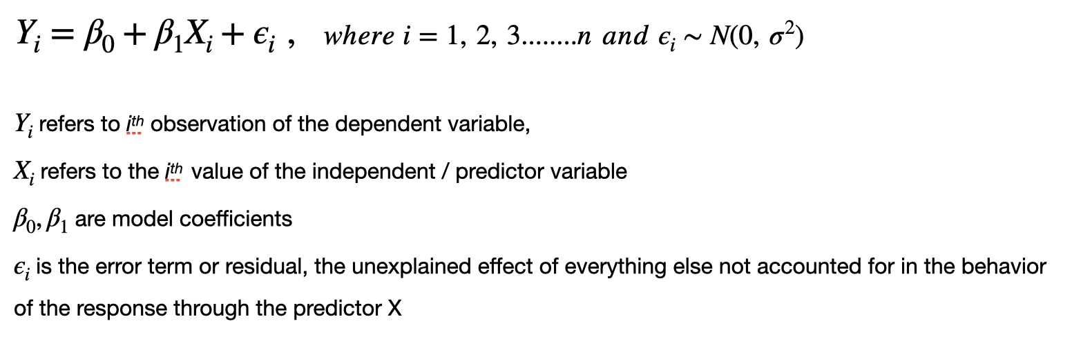
In the case of simple linear regression the model takes the following theoretical form:
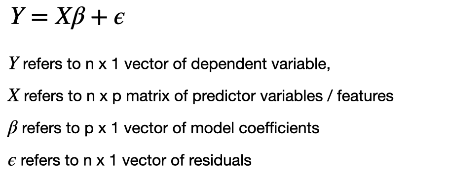
or in matrix form,
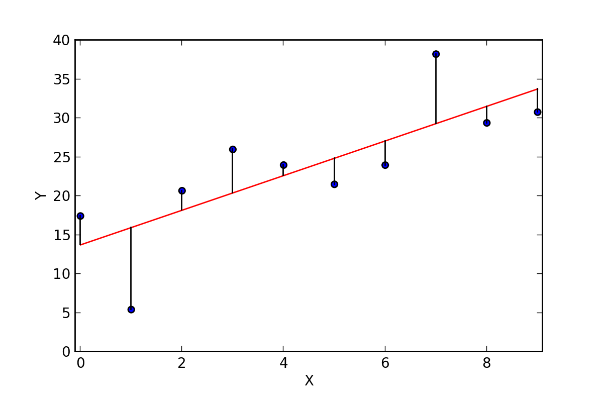
As an illustration of how linear regression works, consider the simple case of one X and one Y variable, of which the relationship between X and Y can be shown on a scatter plot.
Source: Bookdown.org
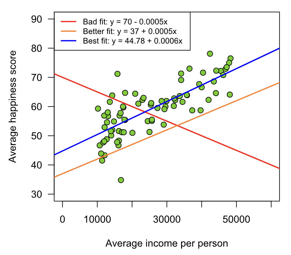
There are infinitely many straight lines that can be drawn through the data points, using different slope and intercept parameters (as shown in the below picture). Many lines would not be a good fit for the data, so the linear regression estimation process finds the slope and intercept (often denoted by 𝞫0 and 𝞫1) that minimizes the variance between the actual y-values and fitted line. The intercept parameter 𝞫0 represents the value of the Y variable when the X variable(s) is set to 0, which only has a meaningful interpretation if 0 is within the naturally occurring range of the X variable. The slope parameter 𝞫1 quantifies the expected change in Y for a 1-unit change in X, where the magnitude of the change is based on the scale of the data as it is estimated by the model. If there are multiple X variables, the interpretation is the same but conditional on all other X variables being held constant, or unchanged, in order to isolate the effect of one variable at a time.
Source: Bookdown.org
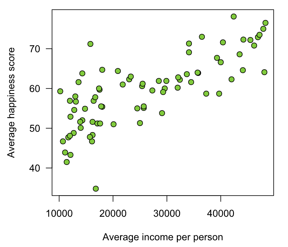
The scatterplot above shows 3 possible choices for regression lines for a given set of data. The red line is clearly a bad fit, since it has a negative slope despite the relationship between X and Y being positive, since as X increases, Y also increases. The orange line is a better fit than the red since it has a slope that appears to closely approximate the general upward trend between X and Y, yet it falls below most of the observations. Finally, the blue line is the best fit of the three, as it passes through the center of the cloud of data, and a similar number of observations lie both above and below the line. The estimation process (usually either Least Squares or Maximum Likelihood) would find the optimal parameters based on minimizing the variance between the predictor(s) X and outcome Y, but this illustration gives some intuition into how the estimation process works.
How are coefficients of linear regression model estimated?
Click here for a detailed answer on estimates of model coefficients
The two most common algorithms for deriving the coefficients of a linear regression model are Ordinary Least Squares (OLS) and Maximum Likelihood (MLE) estimation. In the standard setup of linear regression, where the assumptions of independent, identically distributed (Normal) residuals with constant variance are satisfied, the OLS and MLE estimates are the same.
Ordinary Least Squares (OLS):
After the model is fit, the sum of squared residuals (SSR) is obtained as shown below:
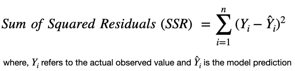
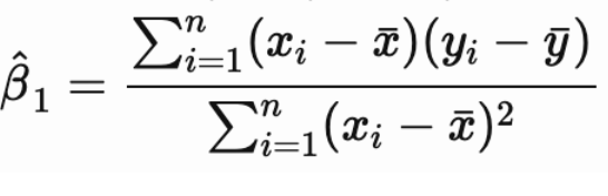
The estimates of the model coefficients are found by taking the partial derivatives of SSR and setting them to 0 to solve what is called the normal equations. In standard matrix form, the OLS solution is written as:
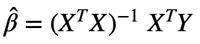
Since this is a closed form solution, the above formula holds true even for higher feature space of X
Maximum Likelihood Estimation (MLE):
Maximum likelihood is a common statistical estimation technique that produces estimates for the coefficients that maximize the likelihood function. The conceptual framework of MLE is that it derives estimates for the parameters that maximize the likelihood of observing the data seen by the model based on its underlying statistical assumptions, which in the case of linear regression, is that the residuals follow a normal distribution with some unknown but constant variance.
Derivation of the MLE estimates for a simple linear regression begins with the likelihood function, L for n independent and identically distributed (iid) observations of a normal distribution, which is mathematically represented by the multiplication of the probability density functions (PDFs) for the said distribution:

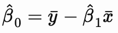
After some algebra and simplification, the MLE estimates for ![]() and
and ![]() can be written as:
can be written as:
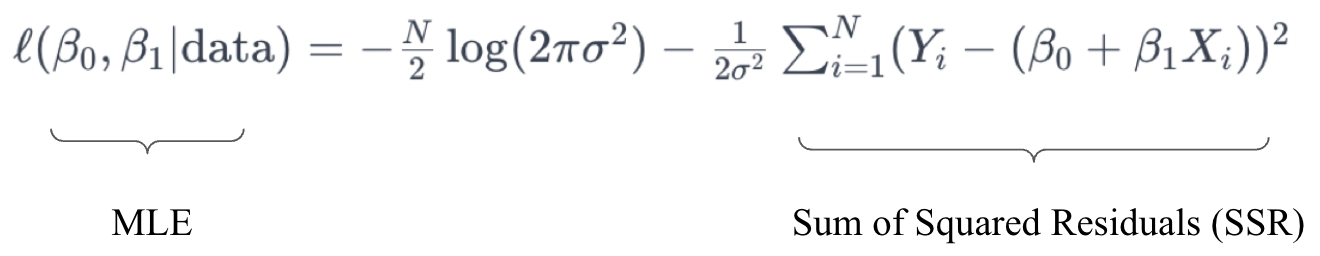
As stated, under the assumptions of linear regression, the OLS estimates and the MLE estimates for the coefficients are equivalent. This equivalency is contingent on the assumption of normally distributed residuals. In the MLE setup, the underlined term on the right hand side of the log-likelihood function is equivalent to the sum of the squared residuals, thus showing the connection to OLS estimation.
Applications of Linear Regression
Linear Regression is a widely utilized technique across all fields and disciplines for modeling the relationship between a continuous dependent variable and one or more predictors. For example:
- Real Estate Pricing: Predicting the selling price of homes based on features such as square footage, number of bedrooms, number of bathrooms, and location
- Stock Market Analysis: Forecasting future stock prices based on historical prices, trading volume, or economic indicators.
- Educational Outcomes: Estimating the impact of study hours, attendance, and prior academic performance on students’ final exam scores.
- Healthcare: Predicting patient outcomes based on clinical variables. For example, a linear regression model could estimate a patient’s blood pressure based on their age, weight, cholesterol level, and smoking status.
- Sales Forecasting: Projecting future sales volumes based on advertising spend, market trends, seasonal factors, and past sales data.
- Energy Consumption: Predicting electricity or gas consumption in households or commercial buildings based on factors like the size of the building, the number of occupants, weather conditions, and the time of year.
- Salary Predictions: Estimating an individual’s salary based on their education level, years of experience, industry, and job role. This can help both employers and employees in salary negotiations and career planning.
Advantages and Disadvantages of Linear Regression
There are both advantages and disadvantages to linear regression. On the positive side, it is probably the most interpretable modeling approach, which gives it an advantage over more modern machine learning techniques when explainability is of high importance. A prediction made by a linear regression model can be explained in full by plugging the values of a given observation into the estimated model equation. For example, if a linear regression model is built to predict GPA using test score, and a student’s test score is 1400, his or her predicted GPA could be found by plugging that value into the equation 𝞫0 + 𝞫1 * 1400, where 𝞫0 and 𝞫1 are the model estimates for the intercept and slope, respectively.
In terms of disadvantages, there are several assumptions that must be satisfied in order to fit a linear regression model on a dataset, and if any of the assumptions are violated, the model likely cannot be used with confidence. Further, in many complex, high-dimensional datasets, a non-linear model is often better suited to uncover the complex relationships present within the data, and linear regression would likely perform worse in comparison to advanced machine learning techniques such as gradient boosting or deep learning.
Video explanation of Regression
Want to learn Regression methods in detail? If so, we recommend the following two lecture series on Regression methods. They are thorough with clear explanations (no affiliations):
- Regression Series by Prof. Justin Zeltzer from University of Sydney (Runtime: 15 mins):
- Regression Modeling for Health Research from Prof. Mike Marin at University of British Columbia (Runtime: 13 mins):
